Appearance
anaconda
在 .bash_profile 中初始化 anaconda
bash
# >>> conda initialize >>>
# !! Contents within this block are managed by 'conda init' !!
__conda_setup="$('/opt/anaconda3/bin/conda' 'shell.bash' 'hook' 2> /dev/null)"
if [ $? -eq 0 ]; then
    eval "$__conda_setup"
else
    if [ -f "/opt/anaconda3/etc/profile.d/conda.sh" ]; then
        . "/opt/anaconda3/etc/profile.d/conda.sh"
    else
        export PATH="/opt/anaconda3/bin:$PATH"
    fi
fi
unset __conda_setup
# <<< conda initialize <<<
验证 conda 命令
bash
conda --versionjupyter
TODO
numpy、pandas 和 matplotlib
TODO
数学基础
微积分
- 推导常见函数的导数:常数、幂函数、指数函数、对数函数和三角函数
- 求导法则
- 二阶导数
- 偏导数:多元函数 多个自变量
- 梯度:多元函数的一组偏导数 上升最快的方向
- 梯度是方向和速率,不是目标点
- 例如:从 (1,1) 出发上升最快的方向是沿着向量(3,3) 指向的方向,而不是指向坐标点 (3,3)
线性代数
- 标量/scalar 向量/vector
- 向量运算:点积/内积/
a @ b/a.dot(y) - (没搞懂)向量范数
- 矩阵运算 转置
概率论
- 概率分布
- 均匀分布/矩形分布
- 伯努利分布
- 二项分布
- 数学期望
- 正态分布/高斯分布
- 期望/均值:μ/谬
- 标准差:σ/西格玛。一定要理解标准差!标准差越大,数据离平均值抖动越厉害,样本差异大;标准差越小,数据围绕平均值紧凑,样本差异小
- 方差:
σ**2/西格玛方 - 标准正态分布:μ=0,
σ**2=1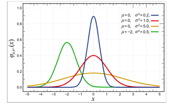
- 随机数常用的三个函数
py
import numpy as np

# 均匀分布 生成 1 个 0 到 1 范围内,随机数
a = np.random.rand()

# 均匀分布 生成 5 个 0 到 1 范围内,随机数
a = np.random.rand(5)

# 均匀分布 生成 1 个 0 到 100 范围内,随机整数
a = np.random.randint(0, 100)

# 均匀分布 生成 shape 为 (2, 3) 的 0 到 100 范围内,随机整数
a = np.random.randint(0, 100, size=[2, 3])

# randn 的 n 表示正态分布,标准正态分布 1 个数
a = np.random.randn()

# randn 的 n 表示正态分布,标准正态分布 10 个数
a = np.random.randn(10)
# a = np.random.randn(10)           # 标准正态 N(0,1)
# b = a * 标准差 + 期望 # 变成 N(期望, 标准差^2)- 贝叶斯定理:先知道结果,然后从结果反推原因发生的概率
- 全概率公式
- 贝叶斯公式
机器学习
- 人工智能、机器学习和深度学习
- 发展历史
- AlexNet ImageNet 李飞飞 CNN
- ILSVRC 比赛(ImageNet Large Scale Visual Recognition Challenge)
- Transformer 使用注意力机制替代 RNN
- 大模型 GPT BERT
- 多模态 CLIP
- 深度学习、强化学习、专家系统
- 量化交易
基本术语
- 特征 标签
- 数据集(训练集 验证集 测试集)
- 验证集用来调整超参数
- 超参数,例如学习率
- 特征向量
特征工程
特征工程主要内容
## **1️⃣ 特征构建(Feature Construction)**

* **核心**:根据原始数据创造新特征,让模型更容易学到规律。
* **方法**:

  1. 数值计算:加减乘除、平方、开方、对数、归一化

     * 例:价格 * 数量 → 总金额
     * 例:log(收入) → 缩小数据尺度差异
  2. 时间特征:年、月、日、工作日/周末、季节

     * 例:电商订单预测 → “周末订单量更高”
  3. 类别组合:类别交叉、频率编码

     * 例:性别 + 地区 → 新特征“男+北上广”
  4. 文本、序列特征提取:TF-IDF、embedding

---

## **2️⃣ 特征选择(Feature Selection)**

* **核心**:挑出有用特征,丢掉没用/噪声的特征。
* **方法**:

  1. **低方差过滤**:方差太小 → 丢掉
  2. **相关性过滤**:和目标相关度低 → 丢掉,和其他特征高度相关 → 也可能丢
  3. **统计检验**:卡方检验、互信息、ANOVA
  4. **模型选择**:Lasso、树模型特征重要性

---

## **3️⃣ 特征编码(Feature Encoding)**

* **核心**:把非数值特征变成数值,模型才能用。
* **方法**:

  1. **独热编码(One-Hot)**
  2. **标签编码(Label Encoding)**
  3. **频率编码 / 目标编码(Target Encoding)**
  4. **嵌入向量(Embedding)** → NLP、类别很多的场景

---

## **4️⃣ 特征缩放 / 标准化(Feature Scaling)**

* **核心**:让特征在同一量纲下,避免模型被尺度大的特征支配。
* **方法**:

  1. Min-Max 缩放 → [0,1]
  2. Z-score 标准化 → 平均值 0,标准差 1
  3. Log / Box-Cox → 异常值处理

---

## **5️⃣ 特征交互(Feature Interaction)**

* **核心**:把两个或多个特征组合成新特征,提高非线性表达能力。
* **例子**:

  * 商品价格 × 用户购买次数 → 总支出
  * 年龄 × 收入 → 消费能力等级
  * 类别组合 → 地区 + 性别 + 渠道

---

## **6️⃣ 特征降维(Feature Reduction)**

* **核心**:减少特征数量,保留核心信息
* **方法**:

  1. PCA、SVD → 线性降维
  2. t-SNE、UMAP → 非线性降维(可视化为主)
  3. Autoencoder → 深度降维
特征选择:低方差过滤法
- 方差:每个数与“平均值”之间差距的平均大小,即这个特征在不同样本之间波动有多大
- 低方差的影响:方差不大,数据都差不多,对预测影响小,模型学不到区分能力
py
import numpy as np
from sklearn.feature_selection import VarianceThreshold

a = np.random.randn(100)
av = np.var(a)
print(f'a的方差:{av}')

# 期望为 5,标准差为 0.1
b = np.random.normal(5, 0.1, size=100)
bv = np.var(b) # 计算方差
print(f'b的方差:{bv}')

X = np.vstack((a, b)).T
# X.shape

# 只保留方差大于 0.01 的特征
vt = VarianceThreshold(threshold=0.01)
X = vt.fit_transform(X)
X.shape
特征选择:相关系数过滤法
两个特征之间的相关性
- 皮尔逊相关系数法
衡量两个变量的线性相关性,取值范围 [-1, 1]
py
import pandas as pd

advertising = pd.read_csv("advertising.csv")
#advertising.head()

# 数据清洗
advertising.drop(advertising.columns[0], axis=1, inplace=True) # 移除索引列
advertising.dropna(inplace=True)
#advertising.head()

X = advertising.drop("Sales", axis=1)
y = advertising["Sales"]
# 计算皮尔逊相关系数
X.corrwith(y, method="pearson")
其它:皮尔逊相关系数矩阵 数据彼此的相关性
- 斯皮尔曼相关系数法
等级变量之间的皮尔逊相关系数,取值范围 [-1, 1]
py
import pandas as pd

# 每周学习时长
X = [[5], [8], [10], [12], [15], [3], [7], [9], [14], [6]]
X = pd.DataFrame(X)

# 数学考试成绩
y = [55, 65, 70, 75, 85, 50, 60, 72, 80, 58]
y = pd.Series(y)

# 计算斯皮尔曼相关系数
X.corrwith(y, method="spearman")
# Output 0.987879
特征降维:PCA
py
import numpy as np
import matplotlib.pyplot as plt
from sklearn.decomposition import PCA
from sklearn.preprocessing import StandardScaler

n_samples = 1000
# 第1个主成分方向
component1 = np.random.normal(0, 1, n_samples)
# 第2个主成分方向
component2 = np.random.normal(0, 0.2, n_samples)
# 第3个方向(噪声,方差较小)
noise = np.random.normal(0, 0.1, n_samples)
# 构造3维数据
X = np.vstack([
    component1 - component2,
    component1 + component2,
    component2 + noise
]).T

# 标准化
scaler = StandardScaler()
X_standardized = scaler.fit_transform(X)
print(f"X_standardized.shape: {X_standardized.shape}")

# 应用PCA,将3维数据降维到2维
pca = PCA(n_components=2)
X_pca = pca.fit_transform(X_standardized)
print(f"X_pca.shape: {X_pca.shape}")

# 可视化
# 转换前的3维数据可视化
fig = plt.figure(figsize=(12, 4))

#ax1 = fig.add_subplot(1, 2, 1, projection="3d") # 1行2列,现在操作第1个
ax1 = fig.add_subplot(121, projection="3d")
ax1.scatter(X[:, 0], X[:, 1], X[:, 2], c="g")
ax1.set_title("Before PCA (3D)")
ax1.set_xlabel("Feature 1")
ax1.set_ylabel("Feature 2")
ax1.set_zlabel("Feature 3")

# 转换后的2维数据可视化
#ax2 = fig.add_subplot(1, 2, 2) # 1行2列,现在操作第2个
ax2 = fig.add_subplot(122)
ax2.scatter(X_pca[:, 0], X_pca[:, 1], c="g")
ax2.set_title("After PCA (2D)")
ax2.set_xlabel("Principal Component 1")
ax2.set_ylabel("Principal Component 2")
plt.show()
模型评估和模型选择
- 库:numpy, pandas, matplotlib, sklearn, torch
- 损失函数
- 使用较多:平方损失函数、对数似然损失函数;使用较少:0-1 损失函数、绝对损失函数
- 平方损失/MSE/均方误差损失函数
- 适用:回归任务
- 形式:
(y − ŷ )²
- 对数似然损失(Log-Likelihood Loss)/对数损失(Log Loss)
- 适用:二分类、多分类
- 核心思想:错误越离谱,惩罚越狠
- 其它损失函数:Lasso / Ridge / Huber / 交叉熵(Cross-Entropy)
- 训练误差、测试误差
- 训练误差/经验误差:模型在“训练数据”上的错误率
- 测试误差:模型在“没见过的新数据”上的错误率
- 模型的泛化能力:
- 拟合(Fitting):训练误差适中、测试误差低
- 欠拟合(Underfitting):训练误差高、测试误差高
- 过拟合(Overfitting):训练误差低、测试误差高
- 欠拟合和过拟合的产生原因
拟合案例
案例:使用多项式在 x 属于 [-3, 3] 上拟合 sin(x)
泰勒展开式
py
import numpy as np
import matplotlib.pyplot as plt
from sklearn.model_selection import train_test_split
from sklearn.linear_model import LinearRegression
from sklearn.metrics import mean_squared_error

def polynomial(X, degree):
  return np.hstack([X ** i for i in range(1, degree + 1)])

# 生成数据集
np.random.seed(7)

X = np.linspace(-3, 3, 300).reshape((-1, 1))
X.shape # (300, 1)

# 基于 sin(x) 叠加随机噪音
y = np.sin(X) + np.random.uniform(-0.5, 0.5, 300).reshape(-1, 1)

fig, ax = plt.subplots(1, 3, figsize=(15, 4))
ax[0].scatter(X, y, c='y')
ax[1].scatter(X, y, c='y')
ax[2].scatter(X, y, c='y')
# plt.show()

# 拆分数据集
X_train, X_test, y_train, y_test = train_test_split(X, y, test_size=0.2)

# 定义模型
model = LinearRegression()

#### 欠拟合

# 训练模型
model.fit(X_train, y_train)
train_loss = mean_squared_error(y_train, model.predict(X_train))

# 测试模型
test_loss = mean_squared_error(y_test, model.predict(X_test))

# 绘制拟合曲线
ax[0].plot(X, model.predict(X), 'r')
ax[0].text(-3, 1, f"Test Loss: {test_loss:.4f}")
ax[0].text(-3, 1.3, f"Train Loss: {train_loss:.4f}")

#### 拟合:将高阶运算转化为多元运算
degree = 5
X_train2 = polynomial(X_train, degree)
X_test2 = polynomial(X_test, degree)

model.fit(X_train2, y_train)
train_loss2 = mean_squared_error(y_train, model.predict(X_train2))

# 测试模型
test_loss2 = mean_squared_error(y_test, model.predict(X_test2))

# 绘制拟合曲线
ax[1].plot(X, model.predict(polynomial(X, degree)), 'r')
ax[1].text(-3, 1, f"Test Loss: {test_loss2:.4f}")
ax[1].text(-3, 1.3, f"Train Loss: {train_loss2:.4f}")

#### 过拟合
degree = 30
X_train3 = polynomial(X_train, degree)
X_test3 = polynomial(X_test, degree)

model.fit(X_train3, y_train)
train_loss3 = mean_squared_error(y_train, model.predict(X_train3))

# 测试模型
test_loss3 = mean_squared_error(y_test, model.predict(X_test3))

# 绘制拟合曲线
ax[2].plot(X, model.predict(polynomial(X, degree)), 'r')
ax[2].text(-3, 1, f"Test Loss: {test_loss2:.4f}")
ax[2].text(-3, 1.3, f"Train Loss: {train_loss2:.4f}")

# 输出模型的参数
print(model.coef_)
print(model.intercept_) # 常数项 b
正则化
- 正则化:给损失函数加一个“惩罚项”,让模型不敢把参数调得太极端,从而减少过拟合
- 正则化技术:
- L1 正则化:绝对值
- L2 正则化:平方
- ElasticNet 正则化:组合 L1 和 L2
- Dropout
- BatchNorm 不是正则化(但会带来正则化效果)
正则化案例
py
ax[1, 2].bar(np.arange(20), ridge.coef_) # 绘制所有系数不是画“模型个数”,也不是画“数据维度”,而是画 w₁, w₂, …, w₂₀ 的数值
交叉验证
TODO
KNN
- KNN 监督学习 工作原理
- KNN 能解决两类问题:分类->投票 和 回归->平均
- KNN 的超参数:K 值
- KNN 的 sklearn API 使用
- KNN 案例:心脏病预测
- 归一化(按比例缩放)和标准化(调整数据分布、正态分布)
- 特征转化:one-hot encoding 多元特征
- 超参数(K 值)调优:网格搜索和交叉验证
线性回归
- 一元线性回归和多元线性回归
- 案例:学习时间和考试成绩的关系
- 线性回归的损失函数
- 均方误差/MSE
- MSE=
1/n * nΣi=1 (y_true - y_pred)**2欧式距离 - 均方误差是回归任务中最常用的损失函数 凸函数处处可导
- 最小二乘法
- MSE=
- 平均绝对误差/MAE
- MAE=
1/n * nΣi=1 |y_true - y_pred|曼哈顿距离
- MAE=
- 均方误差/MSE
- 线性回归的求解
- 最小二乘法求解一元线性回归 -> 求偏导、让偏导为 0、链式法则
- 正规方程法
- 梯度下降法
逻辑回归
- 解决分类问题的方法,特别是二分类
感知机 MLP
- 逻辑门电路:与门、或门、与非门、异或门
- 单层感知机实现与门、或门、与非门
- 多层感知机实现异或门